Newton–Cotes formulas

Newton-Cotes formula for n=2

In numerical analysis, the Newton–Cotes formulae, also called the Newton–Cotes quadrature rules or simply Newton–Cotes rules, are a group of formulae for numerical integration (also called quadrature) based on evaluating the integrand at equally-spaced points. They are named after Isaac Newton and Roger Cotes.

Newton–Cotes formulae can be useful if the value of the integrand at equally-spaced points is given. If it is possible to change the points at which the integrand is evaluated, then other methods such as Gaussian quadrature and Clenshaw–Curtis quadrature are probably more suitable.

Description

It is assumed that the value of a function ƒ defined on [a, b] is known at equally spaced points x_i, for i = 0, …, n, where x₀ = a and x_n = b. There are two types of Newton–Cotes formulae, the "closed" type which uses the function value at all points, and the "open" type which does not use the function values at the endpoints. The closed Newton-Cotes formula of degree n is stated as

$int_a^b f(x) ,dx approx sum_{i=0}^n w_i, f(x_i)$

where x_i = h i + x₀, with h (called the step size) equal to (x_n − x₀) / n = (b − a) / n. The w_i are called weights.

As can be seen in the following derivation the weights are derived from the Lagrange basis polynomials. This means they depend only on the x_i and not on the function ƒ. Let L(x) be the interpolation polynomial in the Lagrange form for the given data points (x₀, ƒ(x₀) ), …, (x_n, ƒ(x_n) ), then

$int_a^b f(x) ,dx approx int_a^b L(x),dx = int_a^b bigl( sum_{i=0}^n f(x_i), l_i(x) bigr) , dx = sum_{i=0}^n f(x_i) underbrace{int_a^b l_i(x), dx}_{w_i}.$

The open Newton–Cotes formula of degree n is stated as

$int_a^b f(x), dx approx sum_{i=1}^{n-1} w_i, f(x_i).$

The weights are found in a manner similar to the closed formula.

Instability for high degree

A Newton–Cotes formula of any degree n can be constructed. However, for large n a Newton–Cotes rule can sometimes suffer from catastrophic Runge's phenomenon where the error grows exponentially for large n. Methods such as Gaussian quadrature and Clenshaw–Curtis quadrature with unequally spaced points (clustered at the endpoints of the integration interval) are stable and much more accurate, and are normally preferred to Newton–Cotes. If these methods can not be used, because the integrand is only given at the fixed equidistributed grid, then Runge's phenomenon can be avoided by using a composite rule, as explained below.

Closed Newton–Cotes formulae

This table lists some of the Newton–Cotes formulae of the closed type. The notation $f_i$ is a shorthand for $f(x_i)$, with x_i = a + i (b − a) / n, and n the degree.

Closed Newton–Cotes Formulae

Degree	Common name	Formula	Error term
1	Trapezoid rule	$frac{b-a}{2} (f_0 + f_1)$	$-frac{(b-a)^3}{12},f^{(2)}(xi)$
2	Simpson's rule	$frac{b-a}{6} (f_0 + 4 f_1 + f_2)$	$-frac{(b-a)^5}{2880},f^{(4)}(xi)$
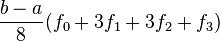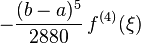
3	Simpson's 3/8 rule	$frac{b-a}{8} (f_0 + 3 f_1 + 3 f_2 + f_3)$	$-frac{(b-a)^5}{6480},f^{(4)}(xi)$
4	Boole's rule	$frac{b-a}{90} (7 f_0 + 32 f_1 + 12 f_2 + 32 f_3 + 7 f_4)$	$-frac{(b-a)^7}{1935360},f^{(6)}(xi)$

Boole's rule is sometimes mistakenly called Bode's rule due to propagation of a typo in Abramowitz and Stegun, an early reference book.

The exponent of the segment size b − a in the error term shows the rate at which the approximation error decreases. The derivative of ƒ in the error term shows which polynomials can be integrated exactly (i.e., with error equal to zero). Note that the derivative of ƒ in the error term increases by 2 for every other rule. The number $xi$ is between a and b.

Open Newton–Cotes formulae

This table lists some of the Newton–Cotes formulae of the open type. Again, ƒ_i is a shorthand for ƒ(x_i), with x_i = a + i (b − a) / n, and n the degree.

Open Newton–Cotes Formulae

Common name	step size	Formula	Error term	Degree
Rectangle rule, or midpoint rule	$frac{b-a}{2}$	$(b-a) f_1,$	$frac{(b-a)^3}{24},f^{(2)}(xi)$	2
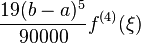
Trapezoid method	$frac{b-a}{3}$	$frac{b-a}{2} (f_1 + f_2)$	$frac{(b-a)^3}{36},f^{(2)}(xi)$	3
Milne's rule	$frac{b-a}{4}$	$frac{b-a}{3} (2 f_1 - f_2 + 2 f_3)$	$frac{7(b-a)^5}{23040}f^{(4)}(xi)$	4
No name	$frac{b-a}{5}$	$frac{b-a}{24} (11 f_1 + f_2 + f_3 + 11 f_4)$	$frac{19(b-a)^5}{90000}f^{(4)}(xi)$	5

Composite rules

For the Newton–Cotes rules to be accurate, the step size h needs to be small, which means that the interval of integration $[a, b]$ must be small itself, which is not true most of the time. For this reason, one usually performs numerical integration by splitting $[a, b]$ into smaller subintervals, applying a Newton–Cotes rule on each subinterval, and adding up the results. This is called a composite rule, see Numerical integration.

See also

• Quadrature (mathematics)
• Interpolation
• Spline interpolation

References

• M. Abramowitz and I. A. Stegun, eds. Handbook of Mathematical Functions with Formulae, Graphs, and Mathematical Tables. New York: Dover, 1972. (See Section 25.4.)
• George E. Forsythe, Michael A. Malcolm, and Cleve B. Moler. Computer Methods for Mathematical Computations. Englewood Cliffs, NJ: Prentice-Hall, 1977. (See Section 5.1.)
• Press, WH; Teukolsky, SA; Vetterling, WT; Flannery, BP (2007), "Section 4.1. Classical Formulas for Equally Spaced Abscissas", Numerical Recipes: The Art of Scientific Computing (3rd ed.), New York: Cambridge University Press, ISBN 978-0-521-88068-8, http://apps.nrbook.com/empanel/index.html?pg=156
• Josef Stoer and Roland Bulirsch. Introduction to Numerical Analysis. New York: Springer-Verlag, 1980. (See Section 3.1.)

External links

• Hazewinkel, Michiel, ed. (2001), "Newton-Cotes quadrature formula", Encyclopedia of Mathematics, Springer, ISBN 978-1-55608-010-4, http://www.encyclopediaofmath.org/index.php?title=p/n066510
• Newton–Cotes formulae on www.math-linux.com
• Newton–Cotes Formulae
• Weisstein, Eric W., "Newton-Cotes Formulae" from MathWorld.
• Module for Newton–Cotes Integration, fullerton.edu
• Newton–Cotes Integration, numericalmathematics.com